This post describes the procedure used to produce post-stratification and country population weights for the CUPESSE data. It provides a short description of the weights available in the dataset, and it describes in detail the procedure used to compute them. Weights have been generated using R version 3.3.2 and the survey package version 3.31-5. Other packages used to write this post are knitr, plyr, and ggplot2.
Weights in the CUPESSE data
The CUPESSE data include four variables for weighting:
-
PWEIGHT_1: Post-stratification weights, to be used for analyses using a single country or multiple countries. It matches the sample to the population based on socio-demographic indicators such as gender, age, education, and region. In Switzerland and Turkey, the question about the level of completed education was not asked to respondents still in education. Hence, to compute PWEIGHT_1, the variable has been imputed for those observations based on the level of education that they will complete (the degree they are currently studying for), their age, and their gender. The imputation procedure is described in detail below, and it affects only Switzerland and Turkey.
-
PWEIGHT_2: Post-stratification weights, analogous to PWEIGHT_1, but computed excluding all the observations in Switzerland and Turkey for which information on the completed level of education is not available (i.e. the respondents who are still in education). In all the other countries, PWEIGHT_2 is identical to PWEIGHT_1.
-
PWEIGHT_IM: Dummy variable identifying the cases in Switzerland and Turkey for which the completed level of education is originally missing, and has been imputed to compute PWEIGHT_1. All the observations with value 1 here are missing in PWEIGHT_2.
-
CWEIGHT: Country population weights, to be used for analysis using multiple countries. It matches the sample size of each country with the country population. It should be used for analyses involving more than one country, when countries are not compared to one another.
The CUPESSE data collection
The CUPESSE project aims to find patterns of individual and family characteristics explaining economic self-sufficiency and entrepreneurial behaviors among European young adults. The countries included in the project are Austria, Czech Republic, Denmark, Germany, Greece, Hungary, Italy, Spain, Switzerland, Turkey, and the UK.
One way in which the project is looking for such patterns is by collecting survey data, and testing quantitative associations between variables. So in 2016, after a common questionnaire had been compiled, each country’s partner institution chose a polling company to conduct the survey, with the goal to interview a sample of at least 1000 young adults (people from 18 to 35 years old) and, for 500 of them, to interview the parents as well.
The survey was conducted online in 9 countries out of 11. Respondents were selected mostly from online panels provided by the polling companies. However, in Hungary and Turkey the poor access to the internet among people living in rural areas required a different strategy. Interviewers had to travel long distances to reach the geographical districts that had been selected in the first stage of sampling. Once there, they had to follow some fixed procedures to select random respondents within the district, and interview them face to face.
Despite the best efforts to obtain samples resembling the reference populations, some groups of people might have been easier to reach than others. This implies that some specific groups might be overrepresented in our data compared to the population, while others might be underrepresented. To reduce this potential source of bias, we produced two sets of survey weights: post-stratification weights and country population weights.
Post-stratification weights
Weights are values that we assign to the observations in our data. They are used when we suspect that our sample does not represent the population too well. When we “weight the data,” we simply tell the software how many times every observation shall be counted when computing aggregate statistics in our data. For instance, if the population consists of 60% females and 40% males, but the sample consists of 40% females and 60% males, we can use a weight that makes the male observations count less and the female observations count more (in this specific case, males will be counted \(\frac{40}{60} = 0.67\) times, and females will be counted \(\frac{60}{40} = 1.5\) times).
Post-stratification weights are used when the distribution of some characteristics in the sample are different from the ones in the population. They can reduce the bias occurring when it is more difficult to reach some groups of people than others (“sampling error”), or when some groups of people are systematically less likely to agree to take the survey than others (“non-response bias”).
Obviously, our sample will never resemble the population perfectly. However, for the CUPESSE project, all we need is our results not to be completely off when we look at indicators like economic self-sufficiency and entrepreneurship. These factors can vary a lot as a function of a few socio-demographic characteristics like gender, age, and education. Moreover, economic conditions may vary dramatically between different geographical areas in the same country. So we will region into account as well. So we compute weights based on these features.
How do we know how the population looks like? Ideally we would use census data. However, censuses are not conducted every year, and populations change. Using census data from 2011 to build weights for a sample collected in 2016 could be even worse than not weighting the data at all. Hence, we follow the strategy of the European Social Survey (ESS) project, and take population data from the European Union Labour Force Survey (LSF). Following ESS, we use two marginal population distributions: one for the cross-classification of gender, age and education (GAE), and the other for region (R).
Aggregate frequencies of these variables in the LFS data are publicly available to everyone via Eurostat. However, given the specific target population of the CUPESSE data (people of age between 18 and 35), we need different age categories from those available on Eurostat. People at the European Statistical Data Support team provided us aggregate frequencies with ad-hoc cutting points for age. We used data for 2015 because, as of February 2017, aggregate data for the last quarter of 2016 were not yet available.
Country population weights
In some cases, we may be interested in showing descriptive statistics for two or more countries together, rather than for a single country. In this case, there is another potential source of bias that we need to take into account: the fact that the country samples in the CUPESSE data are not proportional to the populations of the 11 countries included in the project. For instance, the population of Hungary as of 2015 was 9,844,686 people, and the one of Italy 60,802,085. However, in the CUPESSE data, the sample in Hungary has 1,295 respondents, while the one in Italy 1,008. So in our sample Hungary weighs about 25% more than Italy, while in reality Italy weighs 600% more than Hungary!
This unbalance can be corrected by using country population weights. Such weights have the same value for all observations in the same country, and are useful only when the goal is to show aggregate statistics refrring to the whole CUPESSE sample. To obtain the population frequencies we use data from the World Bank World Development Indicators for the year 2015.
Computing country population weights
Country weigths are the easiest to calculate and the most intuitive to grasp, so we start from them. The first step is to create a table containing the counts that we would observe in each country, if observations in our sample were distributed across countries proportionally to the population. This is necessary because, to calculate weights, the survey package needs to know how the distribution of the different groups in the sample would look like if it resembled the population. Hence, we need to multiply the shares of observations (the relative frequencies) in each country in the population by the total number of observations in the CUPESSE data.
pop.dist <- data.frame(CCODE = c(1040, 1203, 1208, 1276, 1300, 1348, 1380,
                                 1724, 1756, 1792, 1826),
                       pop.totals = c(8611088, 10551219, 5676002, 81413145,
                                      10823732, 9844686, 60802085, 46418269,
                                      8286976, 78665830, 65138232))
pop.dist$Freq <- pop.dist$pop.totals/sum(pop.dist$pop.totals)*nrow(data)
pop.dist
##    CCODE pop.totals      Freq
## 1   1040    8611088  446.0816
## 2   1203   10551219  546.5865
## 3   1208    5676002  294.0348
## 4   1276   81413145 4217.4582
## 5   1300   10823732  560.7035
## 6   1348    9844686  509.9858
## 7   1380   60802085 3149.7401
## 8   1724   46418269 2404.6130
## 9   1756    8286976  429.2915
## 10  1792   78665830 4075.1386
## 11  1826   65138232 3374.3663
The counts show how many observations we would have had in each country if the number of interviews conducted per country was proportional to the country populations. So Austria in 2015 had a population of 8,611,088 people, and to be proportionally represented in the CUPESSE data, given the total number of observations (20,008), Austria should have had only 446 observations. However, in the CUPESSE data Austria has 1,684 observations, which means that to resemble the population, each observation from Austria should be counted \(\frac{446}{1684} = 0.265\) times.
In theory, we could easily calculate country weights by hand by dividing the expected counts (given resemblance to the population) by the observed counts.
pop.dist$Freq/table(data$CCODE)
##
##      1040      1203      1208      1276      1300      1348      1380
## 0.2648940 0.4502360 0.2574736 1.2862026 0.3645667 0.3938115 3.1247422
##      1724      1756      1792      1826
## 1.3168746 0.4284347 1.3511733 1.1232910
However, we will have the survey package doing that for us. This is done with the rake function, which employs a technique called iterative proportional fitting (IPF). IPF is a procedure that, given two different contingency tables, searches for the values to assign to the cells of the first table such that its marginal counts (the row and column “totals”) are the same as in the second table. Conceptually, it can be regarded as a massive game of sudoku, where the goal is to reach some given sums at the end of each row and column. This is achieved by first assigning random values to each cell, and then adjusting them iteratively to meet row and column totals until convergence is reached. This is normally done in a matter of seconds by the software.
# Create a "svydesign" object using "YRESID" to identify individual cases
svy.unweighted.cty <- svydesign(ids = ~YRESID, data = data)

# Use "rake" for the IPF procedure
svy.weighted.cty <- rake(design = svy.unweighted.cty,
                     sample.margins = list(~CCODE),
                     population.margins = list(pop.dist[ ,c("CCODE", "Freq")]))

# Extract "YRESID" and weight values
cweight <- data.frame(YRESID = svy.weighted.cty$cluster,
                      CWEIGHT = weights(svy.weighted.cty))

# Merge them with the CUPESSE data
data <- merge(data, cweight, by = "YRESID", all = T)
The data frame cweight that we created can be merged with the CUPESSE data using YRESID as key. We can now look at the estimated country weights, and compare them with the weights calculated by hand above:
unique(data[, c("CCODE", "CWEIGHT")])
##       CCODE   CWEIGHT
## 1      1040 0.2648940
## 1685   1203 0.4502360
## 2899   1208 0.2574736
## 4041   1276 1.2862026
## 7320   1300 0.3645667
## 8858   1348 0.3938115
## 10153  1380 3.1247422
## 11161  1724 1.3168746
## 12987  1756 0.4284347
## 13989  1792 1.3511733
## 17005  1826 1.1232910
Computing post-stratification weights
Country weights have a single dimension, that is, we only match observations based on their country. However, post-stratification weights are multidimensional: individual observations are being matched based on gender, age, education, and region. This makes it inconvenient to calculate weights by hand, and this is where the survey package becomes very useful.
The first step is to create a table containing the number of observations in the CUPESSE data for each country. This is done for the same reason why we have multiplied every country’s relative share in the population by the total number of observations in the CUPESSE data. Since now weights are going to be calculated separately for each country, we need to know the number of observations in each country.
totals <- data.frame(table(data$CCODE))
names(totals) <- c("CCODE", "total")
We also take the chance to create a variable that matches the ISO numeric codes, used to identify countries in the CUPESSE data, to the so-called “alpha-2” codes, used to identify countries in the LFS data. This will be very useful when the two data sources will be matched.
totals$CCODE <- as.numeric(as.character(totals$CCODE))
totals$CCODE.s[totals$CCODE == 1040] <- "AT"
totals$CCODE.s[totals$CCODE == 1203] <- "CZ"
totals$CCODE.s[totals$CCODE == 1208] <- "DK"
totals$CCODE.s[totals$CCODE == 1276] <- "DE"
totals$CCODE.s[totals$CCODE == 1300] <- "GR"
totals$CCODE.s[totals$CCODE == 1348] <- "HU"
totals$CCODE.s[totals$CCODE == 1380] <- "IT"
totals$CCODE.s[totals$CCODE == 1724] <- "ES"
totals$CCODE.s[totals$CCODE == 1756] <- "CH"
totals$CCODE.s[totals$CCODE == 1792] <- "TR"
totals$CCODE.s[totals$CCODE == 1826] <- "UK"
Data cleaning 1: Gender-Age-Education population frequencies
Here’s an example of how the population data look like:
##   COUNTRY YEAR   AGE HATLEV1D       SEX     VALUE
## 1      AT 2015 18-25    1.Low   1.Males  79.58189
## 2      AT 2015 18-25    1.Low 2.Females  66.78012
## 3      AT 2015 18-25 2.Medium   1.Males 249.28334
## 4      AT 2015 18-25 2.Medium 2.Females 220.08678
## 5      AT 2015 18-25   3.High   1.Males  80.27497
## 6      AT 2015 18-25   3.High 2.Females 125.46554
The key information is contained in the variable VALUE: these are the marginal population frequencies (in thousands of people) estimated by LFS. The goal is to calculate weights so that the relative frequencies of these groups in the CUPESSE data are the same as those observed here.
# Create a variable "CCODE.s" to match the population data with "totals"
gae$CCODE.s <- gae$COUNTRY

# Keep only year 2015
gae <- gae[gae$YEAR == 2015, ]

# Remove "No answer cells for education" (we won't use them)
gae <- gae[gae$HATLEV1D != "No answer", ]

# Calculate population shares
gae <- ddply(gae, .(CCODE.s), transform, SHARE = VALUE/sum(VALUE))

# Recode variables to fit with the data
gae$edu <- ifelse(gae$HATLEV1D == "1.Low", 1,
                  ifelse(gae$HATLEV1D == "2.Medium", 2, 3))
gae$edu.or <- gae$edu # Create an additional education variable
gae$sex <- ifelse(gae$SEX == "1.Males", 1, 2)
gae$age <- ifelse(gae$AGE == "18-25", 1, 2)

# Merge with the country frequencies and compute expected frequencies
gae <- merge(gae, totals, by = "CCODE.s")
gae$freq <- gae$SHARE*gae$total

# Keep only the variables that we need
gae <- gae[, c("CCODE", "sex", "age", "edu", "edu.or", "freq")]
Data cleaning 2: NUTS2 population frequencies
##   COUNTRY YEAR QUARTER   AGE REGION    VALUE
## 1      AT 2016      Q1 15-17     11  8.36093
## 2      AT 2016      Q1 15-17     12 48.16483
## 3      AT 2016      Q1 15-17     13 55.98692
## 4      AT 2016      Q1 15-17     21 17.18311
## 5      AT 2016      Q1 15-17     22 39.47066
## 6      AT 2016      Q1 15-17     31 47.42702
The regional data come with two differences. First the frequencies are broken down by quarter. Second, there are 3 age groups: 15-17 years old, 18-35 years old, and 36+ years old. So we need to do two additional operations: sum all the quarters up to get the year counts, and select only the second age group. Moreover, the data do not come directly with NUTS2 codes, as in the CUPESSE data, but with country codes and separate country specific regional codes. So we need to put together the COUNTRY and REGION variables to generate NUTS2 codes that are compatible with the survey data.
# Create a variable "CCODE.s" to match the population data with "totals"
region$CCODE.s <- region$COUNTRY

# Keep only year 2015
region <- region[region$YEAR == 2015, ]

# Keep only people in the "18-35" age group
region <- region[region$AGE == "18-35", ]

# Generate NUTS2 codes
region$YNUTS2 <- paste0(as.character(region$CCODE.s),
                        as.character(region$REGION))
region$YNUTS2 <- gsub("GR", "EL", region$YNUTS2)

# Remove NUTS2 units that are not in our data
region <- region[which(region$YNUTS2 %in% unique(data$YNUTS2)), ]

# Put the 4 quarters together
region <- ddply(region, .(CCODE.s, YNUTS2), transform,
                VALUE.TOT = sum(VALUE))
region <- region[region$QUARTER == "Q1",] # Keep only one quarter

# Calculate population shares
region <- ddply(region, .(CCODE.s), transform,
                SHARE = VALUE.TOT/sum(VALUE.TOT))

# Merge with the country frequencies and compute expected frequencies
region <- merge(region, totals, by = "CCODE.s")
region$freq <- region$SHARE*region$total

# Keep only the variables that we need
region <- region[, c("CCODE", "YNUTS2", "freq")]
Data cleaning 3: CUPESSE data
In this part we need to clean the variables on gender, age, education and region in the CUPESSE data, to match them with the population frequencies.
Gender
1 = Male; 2 = Female
data$sex <- data$YQ42
Age
1 = 18-25 years old; 2 = 26-35 years old (removing the few cases where we don’t have a response)
data$age <- ifelse(data$YQ1 >= 18 & data$YQ1 <= 25, 1,
                   ifelse(data$YQ1 > 25, 2, NA))
Education
1 = Low education (ES-ISCED categories 1–2, up to lower secondary education completed); 2 = Medium education (ES-ISCED categories 3–5, higher secondary and post-secondary, non-tertiary education); 3 = High education (ES-ISCED categories 6–7, post secondary education).
data$edu.or <- NA
data$edu.or[data$YQ18_II == 1 | data$YQ18_II == 2] <- 1
data$edu.or[data$YQ18_II == 3 | data$YQ18_II == 4 | data$YQ18_II == 5] <- 2
data$edu.or[data$YQ18_II == 6 | data$YQ18_II == 7] <- 3
Here we have a problem: in Switzerland and Turkey, the variable YQ18_II (level of completed education) is missing for all the respondents who are still in education. This is visible by looking at the number of missing observations in the newly created edu.or variable in each country. (The country codes for Switzerland and Turkey are 1756 and 1792 respectively).
##       CCODE
## edu.or 1040 1203 1208 1276 1300 1348 1380 1724 1756 1792 1826
##   1     154  135   79  264   28  199   42  431   32  977  449
##   2    1021  652  667 1855  612  863  480  734  300  836 1202
##   3     475  427  370 1134  898  233  486  661  301  501 1353
##   <NA>   34    0   26   26    0    0    0    0  369  702    0
Since we have no information about the degree that they achieved, it is not possible to calculate weights for those respondents–unless we find some surrogate information that we can use. Fortunately, the CUPESSE data also include the variable YQ18_I which records, for those still in education, the degree that they will complete. This, together with age and gender, should be a good enough predictor of the level of education that the respondents have already completed. We can therefore use these variables to “guess” a plausible educational category for the respondents currently in education for which YQ18_II was not observed, and calculate weights based on this.
The procedure is as follows. First, we recode all variables as necessary. Second, we estimate an ordinal logistic regression model to obtain the effects of the degree to be completed, age, and gender on the completed level of education coded in 3 categories (Low, Medium, High). All predictors are treated as categorical, so for instance, the effect of age is not estimated linearly, but separately for each year. This allows to maximize the model fit and therefore its predictive power. The model is estimated on a pooled sample consisting of all countries besides Switzerland and Turkey.
Of course, one could argue that the effect of the predictors may change from country to country, therefore our estimated coefficients may not generalize to the two countries for which we want to obtain predictions. This is definitely a concern, however there are no reasons to expect a systematic difference between Switzerland and Turkey on one side, and all the other countries in the project on the other. In other words, we can assume our model to be as good (or as bad) in Switzerland and Turkey as it is elsewhere.
Finally, we predict the completed level of education based on respondents’ gender, age, and degree to be completed. We can have a look at how well our model predicts the data by comparing the observed level of completed education (the dependent variable in the ordinal model) with the one predicted using the model parameters. The model produces predictions that are correct in 76% of the cases–not perfect, but not too bad either, given that by pure chance we should be able to correctly predict the outcome in 33% of the cases. The full code to replicate the procedure can be found here.
To see the effect of this operation, we can compare the variable edu.or computed above based on YQ18_I with the variable edu, where the missing cases in Switzerland and Turkey have been imputed using the procedure above.
xtabs(~ edu + CCODE, data, exclude = NULL, na.action = na.pass)
##       CCODE
## edu    1040 1203 1208 1276 1300 1348 1380 1724 1756 1792 1826
##   1     154  135   79  264   28  199   42  431   58  980  449
##   2    1021  652  667 1855  612  863  480  734  365 1476 1202
##   3     475  427  370 1134  898  233  486  661  579  512 1353
##   <NA>   34    0   26   26    0    0    0    0    0   48    0
Note that in edu, the missing observations in Switzerland and Turkey are substantially less than in edu.or–in fact, only 48 missings are left in Turkey, which are usual non-responses. So we can calculate our weights based on the variable edu, which allows to retain as many observations as possible.
Region
Just removing missing observations and the possible white space from the NUTS2 codes (recommended with string variables).
data$YNUTS2 <- ifelse(data$YNUTS2 == "-99", NA, data$YNUTS2)
Computing the weights
We can now use the functions in the survey package to compute the weights based on the GAE+R marginal frequencies. We compute the weights separately for each country, so the procedure is done in a loop.
Since education has been imputed for some observations, we generate weights based on both the original data, with a lot of missing observations (using the variable age.or) and the data with education imputed for respondents in education in Switzerland and Turkey (using the variable age).
One important point regards the need to trim the weights. Sometimes the IPF procedure produces weights that are way too big or too large. This happens when the sample marginals are way off compared to the population marginals, i.e. some groups (e.g. male of age between 18 and 25 with high level of education) have too few or too many observations with respect to the population. Trimming weights implies setting an arbitrary threshold so that all smaller and larger weights are collapsed to its lower and higher boundaries. This produces some small bias in the weights, but having observations that are counted e.g. 20 times is not that good either. Following ESS we set only the upper threshold at 4.
# Generate two data sets excluding all missing observations in the variables
# used for weighting
data.2 <- data[!is.na(data$YNUTS2) & !is.na(data$sex) & !is.na(data$age) & !is.na(data$edu), ]
data.3 <- data[!is.na(data$YNUTS2) & !is.na(data$sex) & !is.na(data$age) & !is.na(data$edu.or), ]

# Generate two empty data frames where to store the weights
pweight <- data.frame(NULL)
pweight.or <- data.frame(NULL)

# Loop over countries
for (i in unique(data$CCODE)){

  # Select the country in the population data
  region.loop <- region[region$CCODE == i, c("YNUTS2", "freq")]
  gae.loop <- gae[gae$CCODE == i, c("sex", "age", "edu", "freq")]
  gae.loop.or <- gae[gae$CCODE == i, c("sex", "age", "edu.or", "freq")]

  # Select the country in both versions of the CUPESSE data
  svy.unweighted <- svydesign(ids = ~YRESID,
                              data = data.2[data.2$CCODE == i, ])
  svy.unweighted.or <- svydesign(ids = ~YRESID,
                                 data = data.3[data.3$CCODE == i, ])

  # Calculate weights
  svy.weighted <- rake(design = svy.unweighted,
                       sample.margins = list(~YNUTS2, ~sex + age + edu),
                       population.margins = list(region.loop, gae.loop))
  svy.weighted.or <- rake(design = svy.unweighted.or,
                          sample.margins = list(~YNUTS2, ~sex + age + edu.or),
                          population.margins = list(region.loop, gae.loop.or))

  # Trim weights at 0.3 and 3
  svy.rake.trim <- trimWeights(svy.weighted, upper = 4,
                               strict = T)
  svy.rake.trim.or <- trimWeights(svy.weighted.or, upper = 4,
                                  strict = T)

  # Put them together
  pweight <- rbind(pweight,
                   data.frame(CCODE = i,
                              YRESID = svy.weighted$cluster,
                              PWEIGHT_1 = weights(svy.rake.trim)
                              )
                   )
  pweight.or <- rbind(pweight.or,
                      data.frame(YRESID = svy.weighted.or$cluster,
                                 PWEIGHT_2 = weights(svy.rake.trim.or)
                      )
  )

  # Remove objects that we don't need anymore to avoid stuffing the memory
  rm(region.loop, gae.loop, gae.loop.or)
  rm(svy.unweighted, svy.unweighted.or)
  rm(svy.weighted, svy.weighted.or)
  rm(svy.rake.trim, svy.rake.trim.or)
}

# Merge the two sets of weights
pweight <- merge(pweight, pweight.or, by = "YRESID", all = T)

# Put a dummy variable to identify imputed observations
pweight$PWEIGHT_IM <- ifelse(is.na(pweight$PWEIGHT_2) &
                               !is.na(pweight$PWEIGHT_1), 1, 0)

# Merge the weights with the CUPESSE data
data <- merge(data, pweight, by = c("YRESID", "CCODE"), all = T)
Comparing weights with and without imputed education
Let us compare the weights computed imputing the achieved degree to those who are in education in Switzerland and Turkey to those computed without imputation. Obviously the transformation won’t affect other countries, but in the two countries where the imputation was conducted, all the other observations will be affected as well (due to the IPF procedure). But to what extent?
Looking at the Pearson’s correlation between the two weights, the values look good: 0.89 in Switzerland and 0.87 in Turkey. We can also plot the two weights against each other in both countries, and inspect their correlation visually.
ggplot(subset(data, CCODE == 1756 | CCODE == 1792),
       aes(x = PWEIGHT_2, y = PWEIGHT_1)) +
  geom_abline(aes(intercept = 0, slope = 1)) +
  geom_point(aes(col = factor(edu))) +
  facet_wrap(~CCODE) +
  scale_x_continuous(limits = c(0, 4)) +
  scale_colour_manual(values = c("blue", "red", "black"),
                      labels = c("Low", "Medium", "High"),
                      "Level of education") +
  xlab("Without imputation") +
  ylab("With imputation") +
  theme_bw()
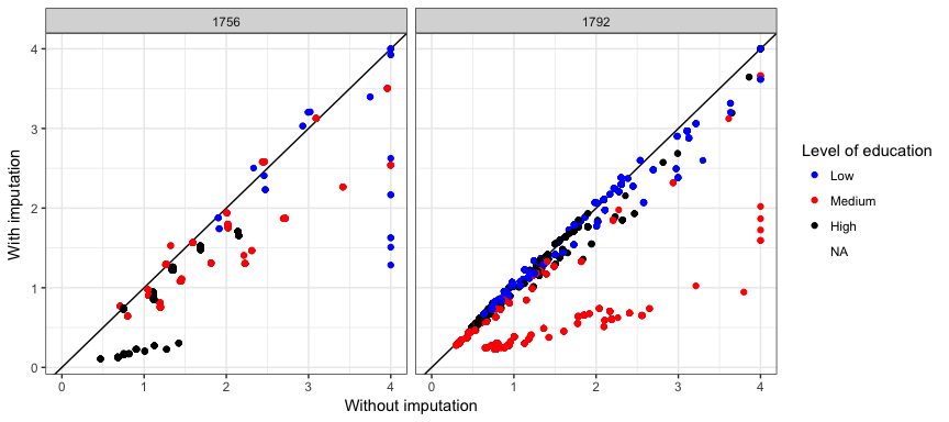
As expected the weights tend to have smaller values when using imputation, because by doing so we increase the counts in all cells. In general, the cases where we observe greater differences are the extreme categories (“Low” and “High”) in Switzerland, and the “Medium” category in Turkey.